Why Censoring?
Censoring occurs in almost every survival analysis and therefore an understanding of it is essential if you wish to be able to interpret survival analyses. We were introduced to the concept in the basic survival analysis post. Let’s review how and why it can occur.
We saw in the basics post that censoring occurs when we don’t know the exact time of the occurrence of the event of interest and for one of three reasons:
- The event of interest doesn’t occur during the study period
- The subject leaves the study before the event occurs
- The subject is ‘lost to follow-up’ which just means that the subject left the study at some point without telling anyone.
Now let’s delve a little deeper into the concept.
There are three main types of censoring: right, left, and interval. To illustrate this, let’s imagine an example.
Suppose I’m a fisherman who wants to explore survival analysis (a bad fisherman probably, as this wouldn’t be a good way to fish), and I’m interested in the the time it takes to catch a fish from my favorite fishing location. I set up 4 poles, each made so they can stand up on their own so I can leave them unattended. I cast all the lines out and plan monitor the time it takes until I catch a fish, but I only have 5 hours total to fish. Being a typical fisherman 😉 I decide that I’ll go have a beer at a nearby beach bar and return only every hour to check on the fishing poles.
So let’s review: the event of interest is catching a fish. The subjects are the poles. The time is time in hours (only checked each hour since I’m busy having a beer), and the study duration is 6 hours.
After the study is over, I’ve got my data collected from checking on the fishing poles every hour. Here’s my dataset:
| pole | surv_time | fish_caught |
| 1 | 2 | 1 |
| 2 | 6 | 0 |
| 3 | 3 | 0 |
| 4 | 1 | 1 |
I’ve got my 4 poles, the survival time in hours, and whether not I caught a fish. With pole 1 I caught a fish, and noticed that this occurred at hour 2. Here, the true time of catching the fish is between 1 and 2 hours, since at hour 1 I did not observe a caught fish; it could have occurred any time after the hour 1 check up to the hour 2 check. The is called interval censoring. The true survival time is within a known interval.
With pole 2, I did not catch a fish, but I had to go home at hour 6 (the study ended). So the true survival time is greater than 6, but I won’t know it, as the study ended. This is an example of right censoring, because the true occurrence of the event of interest is or would be later than a certain time.
Another example of right censoring occurred with pole 3. Let me explain what happened. I returned at hour 3 to check the poles. To my surprise, pole number 3 had disappeared. I have no idea what happened to it. I looked around for it, even asked some people back at the bar, but could not locate it. I don’t know if I caught a really big fish or if someone took the pole or it disappeared for some other reason. Pole 3 is also right censored because the event could have occurred after a certain time, not because the study ended, but rather because the pole was lost-to-follow-up.
The Effects on the Survival Curves
Now that we understand the basics types of censoring, lets look at how it affects the Kaplan-Meier survival curve. Remember from the previous post I mentioned that the calculation becomes more complicated when we have censored data? This calculation:

or

So what do we do when we have censored data?
Let’s go back to the ‘anderson’ dataset from the Survival Analysis Basics post and look more closely at the calculation of the survival curve for the Rx=0, or the new treatment group. In this group there is censoring. In that post you saw the survival object vector, calculated in R, as: 35+ 34+ 32+ 32+ 25+ 23 22… These are the survival times in weeks. A + after the number of weeks means that this subject was censored. These are also displayed in the plot of the survival curves. The + sign is just the accepted way to signify a censored data point.
Now, how do we take the censored data points into account when calculating the survival proportion? Look at the summary for the survival curve for Rx=0:
| time | n.risk | n.event | survival |
| 6 | 21 | 3 | 0.857 |
| 7 | 17 | 1 | 0.807 |
| 10 | 15 | 1 | 0.753 |
| 13 | 12 | 1 | 0.69 |
| 16 | 11 | 1 | 0.627 |
| 22 | 7 | 1 | 0.538 |
| 23 | 6 | 1 | 0.448 |
If we use our original equation, we can start the calculation. Remember, we have 21 subjects in this group. At time = 6, 3 subjects had the event of interest occur (this is from the n.event variables which records the number of events at each time). So (21-3)/21 = 0.857 This looks good, it corresponds with the calculation done by R above. Let’s check the next one when one more event occurred. (21-3-1)/21 = 0.8095. Uh oh. That’s a bit off. You will see the next calculation is a little off as well. What happened? Censoring. Look back at the table above. The n.risk column shows the number of subject at risk for the event to occur. At time = 6, there were 21 subject at risk, the total number at the start of the study. And at time = 6, 3 events occurred. Then at time = 7, one event occurred but now it says there are 17 subjects at risk. Huh? 21-3 ≠ 17, it equals 18. So shouldn’t the n.risk at time = 7 be 18? Nope, we’ve got a censoring issue.
Let’s go back to the original data. Here’s a table of just the events when time = 6 for the new treatment group. Remember, relapse is the event of interest.
| subject | surv_time | relapse | sex | log_WBC | Rx |
| 18 | 6 | 0 | 0 | 3.2 | 0 |
| 19 | 6 | 1 | 0 | 2.31 | 0 |
| 20 | 6 | 1 | 1 | 4.06 | 0 |
| 21 | 6 | 1 | 0 | 3.28 | 0 |
Ah, there are four subjects for time = 6. But above, there were only 3 events. Yes, that is correct. There are 3 subjects at time = 6 who had the event occur. And one who didn’t. This subject was censored. He must have been lost-to-follow-up like the fishing pole I couldn’t find in our fishing study above.
Great, now we know what happened, but how do we change the calculation so that we get the correct survival proportion at week 7?
At time = 0, the survival proportion is 1 or (21/21). Look at the survival curve table above. The survival proportion, the ‘survival’ column starts at 0.857, or 18/21. Then it reduces to 0.807, a 0.05 difference. We started with 21 subjects so our n.risk is 21. Then at time = 6, 3 subjects had the event occur. So 18/21 = 0.857 is our survival proportion. No problem.
But we’ve lost a subject. Look at week 7. Our n.risk states that we have 17 subjects at risk. This is from the number of subject at risk from the previous week, 21, minus the number who had the event occur, 3, AND the number who left the study, 1. 21-3-1 = 17. So the number of subjects at risk at week 7 is 17. We have 1 event at week 7, so (17-1)/17 = 0.941. But that’s not correct. The survival proportion should be 0.807 at week 7.
Here’s what we do: we have to multiply the 16/17 proportion by the previous proportion. Think of it as a proportion of a proportion. 0.857 * 0.942 = 0.8066. Not exactly what we have above, but that’s just due to rounding 0.8066 to 0.807.
For the next survival proportion at time = 10, we multiply the number at risk at time = 10, which is 15. At time = 7, we saw that 1 event occurred. There were 17 subjects at risk so we must have had another subject who left the study. If you look at the original data, you will see that this did happen. At time = 10, 1 event occured. 14/15 = 0.93333. As before, we must multiply this by the previous survival proportion. 0.9333 * 0.0857 = 0.753 Same as in the survival table above!
Now let’s generalize and rewrite the equation.

The important changes are the inclusion of the proportion at t-1 (the previous time’s proportion) and the ‘subjects at risk’ instead of total subjects.
The Kaplan-Meier Curve Revisited
Now we can look at the plot of the survival curve. It’s the same one we saw in the basics of survival analysis post.
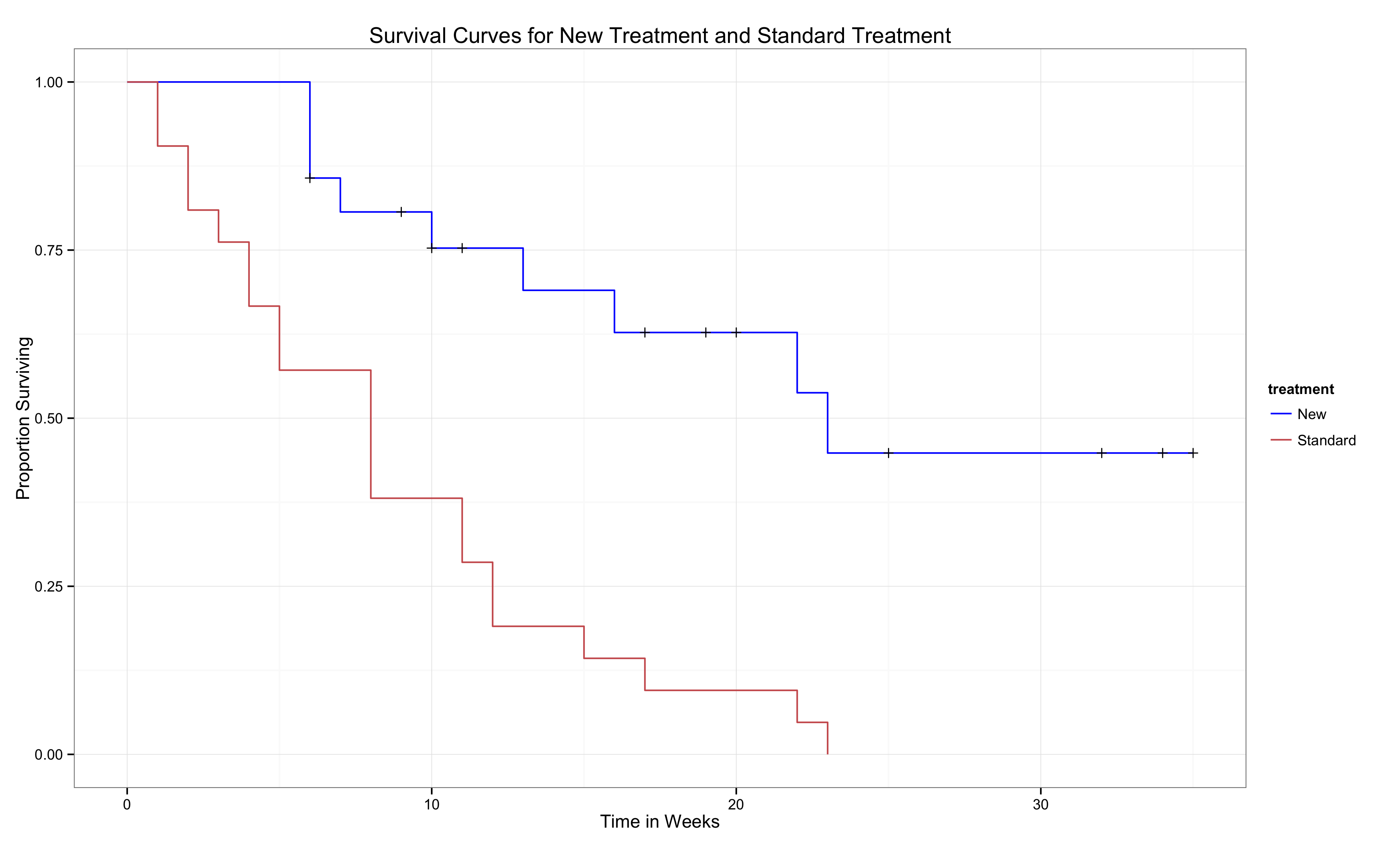
See the + signs? That’s a censored data point. Notice how the curve does not always drop when we encounter one. It only drops when we encounter an event of interest. Then we use the censoring information to calculate the survival proportion. Sometimes an event of interest and censoring occur at the same time, like in week 6. Just note that the censored data only affects the survival curve when an event of interest occurs after the censoring.
Is It Over Yet? That must be all I need to know about censoring.
That was quite a long and dense post. If you’ve gotten this far, I’m impressed. So, are we through with censoring? Nope! That’s just the beginning. The analysis of survival data with censoring can become very complicated especially when performing statistical tests on the data. Luckily whatever software you use will usually deal with the complicated calculations. It is however, necessary to have an idea of what’s going on under the hood. That way, we can understand and critique the results of our analyses in a more effective way.
We’ll definitely see censoring in future posts. But I think that will do it for the introduction to censoring.
At least we caught some fish!

One thought on “Survival Analysis: Censoring”