Ok, so we have gone over the basics and censoring. Now let’s look at how to really tell whether two survival curves are different. In the previous posts we looked survival curves from a leukemia dataset, comparing a new and standard treatment. It was pretty clear when we plotted the curves that there was a difference. But what do we do if the visual analysis is not enough to determine a difference? Or if we want a more statistically valid way analyzing the difference?

We must turn to a statistical test. In this post, we’ll learn how to analyze two survival curves with the Log-rank test.

Take a look at these survival curves from a different dataset, regarding survival times of patients with a certain kind of liver disease.

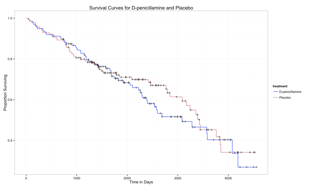
What do we notice? First, notice the title: Suvival Curves for D-penicillamine and Placebo. Second, the axes: time in days and proportion surviving. Then the legend: D-penicillamine and Placebo. So it looks like a normal survival curve plot, comparing two treatments. But in this one it’s not clear if D-penicillamine (treatment) or placebo (no treatment) is better. Note a few interesting features of the curves: 1) there’s a lot of censored data 2) the curves overlap each other, sometimes one is higher, then the other is higher 3) at the end, it appears that the treatment leads to lower survival times than does no treatment.

Would you take the treatment?

Yeah, I probably wouldn’t either. But lets make this analysis more statistically valid.

There will be some new terminology but bear with me as they will be explained briefly here and in more detail in a future post.

The Log-Rank Test

This is a widely used test and the “most popular method of comparing the survival of groups” in clinical studies when we wish to analyze survival or time to event data. It is a hypothesis test which means that we must first state what our null hypothesis is, and what the alternative to this hypothesis is. We will, with the help of statistical software, compute a p-value to determine whether we can fail to reject the null hypothesis or reject the null hypothesis. The p-value is computed by comparing the observed versus the expected number of events for each time period. This difference for each time period is added up to get the log-rank statistic. This statistic is χ² distributed so we can compare it to a χ² distribution to determine the p-value. Then we can either reject or fail to reject the null hypothesis depending on the size of the p-value.

What? Has your survival time just now been left-censored?!!

Don’t leave before we begin! You’ll understand these terms soon (or at least not run away from them). Let’s take a look at them briefly. More will be written on them later, or feel free to Google them.

Null Hypothesis: 

The ‘conservative’ or default position, no difference between treatments (or whatever you are testing). Our null hypothesis would be: There is no difference between the two survival curves, i.e. no difference between the placebo and D-penicillamine treatment.

Alternative Hypothesis:

Yes, literally the alternative to the null hypothesis. There is a difference between treatments. Usually this is what a researcher hopes will occur, e.g. test of a new drug vs. standard treatment. The researcher would like the data to support alternative hypothesis. This can lead to problems and biases…another subject.

Fail to reject or reject the null hypothesis:

Sorry, that’s how we word the conclusion of statistical tests. Either we fail to reject, or we reject the null hypothesis. We NEVER accept the null or alternative hypothesis or prove that it is true or false. Do not even say that. It’s akin to statistical blasphemy. (ok that’s a bit extreme…there are entirely different kinds of…nevermind)

χ² Distribution (Chi-squared)

Pronounced like “kigh” to rhyme with high. This is the difficult one for the less mathematically inclined. I’ll just say that it’s best to think of it as a sort of reference distribution for this statistical test. We compute the log-rank statistic (some number) and compare it with the Χ² distribution with the correct degrees of freedom. Sorry for the Wikepedia links, but it would too long to explain all that here.

P-value

The all-important p-value. It’s a probability (0 to 1). The textbook definition is: “the probability, under the assumption of the null hypothesis, of obtaining a result equal to or more extreme than what was actually observed.” It’s sort of like a standardized way to interpret results of statistical tests. A result is usually deemed ‘statistically significant’ if the p-value is less than 0.05. If it is less than 0.05, we say that we ‘reject the null hypothesis at a 0.05 significance level.’ Why 0.05? It’s just what most scientists have concluded to be a reasonable level of significance. This will definitely be the subject of a future post.

Observed Number of Events

This is just the observed number events of interest (survival events) in our dataset.

Expected Number of Events

This one is a bit tricky. How can we get an expected number of events from our dataset? Remember our null hypothesis: There is no difference between the two survival curves. That is what we ‘expect’ to happen. We expect the null hypothesis. We expect the two survival curves to be the same. (the idea is that this reduces bias towards the alternative hypothesis) So the expected number of events is a sort of average between the two, calculated each time an event of interest occurs. The difference between the so-called average and the observed number of events is calculated for each group. The difference at each event occurrence is added up, and this is the log-rank statistic. If the average survival curve is far from the actual curves, the log-rank statistic will be large. Conversely, if the average survival curve is close to the actual curves, the log-rank statistic will be small. I won’t go through the specific mathematical steps to calculate the statistic. It’s enough to have cursory idea of how it’s done, unless you want to get a degree in statistics!

So, don’t worry, this calculation is done quickly and painlessly in R, or any other statistical software. And once we have the log-rank statistic, we can calculate the p-value (well, R can calculate it).

The Software Output

We’ll see the entire R-code to load the data, create the plot and perform the log-rank test at the end of the post.

The output for the log-rank test will look something like this:

	N	Observed	Expected	(O-E)^2/E	(O-E)^2/V
penicillamine=1	136	57	53.7	0.209	0.405
penicillamine=2	140	54	57.3	0.195	0.405
	Chisq=0.4	on 1 degree	of freedom,	p = 0.525

The most important thing to note here is the p-value. It is 0.525. Remember I stated earlier that a p-value of less than 0.05 is deemed to be statistically significant. 0.525 is much larger than 0.05 so we do not reject the null hypothesis. Instead, we fail to reject the null hypothesis that the treatments are different.

Also note the Chisq=0.4. This is our log-rank statistic. It’s very small, which means that the ‘average’ survival curve was very close to the actual curves. The Chisq distribution with 1 degree of freedom is our ‘reference distribution.’

Conclusion

Here’s a nice way to write the conclusion.

The log-rank test on our data, comparing the survival curves of the placebo to the D-penicillamine treatment, resulted in a p-value of 0.525. Thus, we fail to reject the null hypothesis at a 0.05 level of significance. The data support the claim that the D-penicillamine treatment is no better than placebo.

In short, don’t take the drug.

The Data

The data comes from the University of Massachusetts dataset repository.  There are a lot of survival datasets you can play around with there. The one we analyzed above involves patients at the Mayo Clinic with primary biliary cirrhosis (PBC) of the liver. For the above illustration, I used the D-penicillamine treatment to compare variable to group the patients.

The R-code

The R-code to produce the plot is very similar to that of the Survival Analysis Basics post so I won’t go through it line by line.

To perform the log-rank test we just need to add one more line of code.

survdiff(Surv(surv_time, death==1) ~ penicillamine, data=pbc_comp)

This performs the log-rank test and produces the table seen above.

Yup, add one line of code and a whole new blog post is needed!

Ok, actually there’s one more line of code added, but just to remove the subjects with missing data. The following line removes the patients with missing data. The R function ‘complete.cases’ returns a logical vector (true or false) indicating complete or missing data. This line tells R to take only the cases in the data frame pbc without missing data.

pbc_comp = pbc[complete.cases(pbc), ]

Here’s all of the R-code.

library(GGally)
library(survival)
library(ggplot2)

pbc=read.table("https://www.umass.edu/statdata/statdata/data/pbc.dat",na.strings = ".",
col.names=c("id","surv_time","death","penicillamine","age","sex","ascites","hepatomegaly","spiders","edema","bilirubin","cholesterol","albumin","urine_copper","alk_phosph","SGOT","Triglycerides","platelets","prothrombin_time","disease_stage"))

pbc_comp = pbc[complete.cases(pbc), ]

pbc_comp$SurvObj = with(pbc_comp, Surv(surv_time, death == 1))

pbc_surv = survfit(SurvObj ~ penicillamine, data = pbc_comp)
summary(pbc_surv)

p = ggsurv(pbc_surv,cens.col="black")+theme_bw()+xlab("Time in Days")+ylab("Proportion Surviving")+
  ggtitle("Survival Curves for D-penicillamine and Placebo")
p = p+  guides(linetype = FALSE) 
p = p+ scale_colour_manual(
  name   = 'treatment',
  breaks = c(1,2),values=c("blue","indianred"),
  labels = c('D-penicillamine', 'Placebo'))+theme(legend.key = element_blank())
p

ggsave("surv_plot.png",scale=1.2)


survdiff(Surv(surv_time, death==1) ~ penicillamine, data=pbc_comp)